Table of Contents
Introduction
The LTRpred package implements a software pipeline and provides an integrated workflow to screen for intact and potentially active LTR retrotransposons in any genomic sequence of interest. For this purpose, this package provides a rich set of analytics tools to allow researchers to quickly start annotating and explore their own genomes.
The de novo prediction of LTR transposons in LTRpred is based on the command line tools LTRharvest and LTRdigest and extends these search strategies by additional analytics modules to filter the search space of putative LTR transposons for biologically meaningful candidates.
Please make sure that all command line tools are installed properly before running any LTRpred function.
Getting Started
The rationale for implementing LTRpred was to implement an R based pipeline combining the most sensitive, accurate, and conservative state-of-the art LTR retrotransposon detection tools and extend their inference by additional analyses and quality filtering steps to screen for functional and structurally intact elements. Hence, LTRpred aims to provide a high-level de novo prediction infrastructure to generate high quality annotations of intact LTR retrotransposons. All LTRpred functions are generic so that parameters can be changed to detect any form of LTR retrotransposon in any genome.
Internally, LTRpred is based on the de novo annotation tools LTRharvest and LTRdigest which use prior knowledge about DNA sequence features (also referred to as Structure-based methods) such as the homology of Long Terminal Repeats (LTRs), Primer Binding Sites (PBS), gag and pol protein domains, and Target Site Duplications (TSDs) that are known to enable the process of transposition (Bergman and Quesneville, 2007) to infer LTR retrotransposons in any genome.
Hence, these de novo annotation tools are designed to screen the genome systematically and efficiently for these structural DNA features. Figure 1 shows the structural features of LTR retrotransposons that are used for predicting putative LTR transposons de novo in any genome of interest.
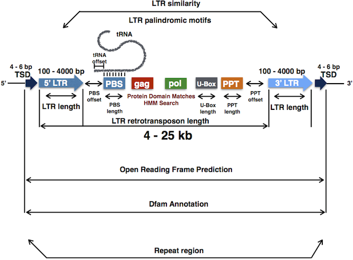
Sequence features of LTR retrotransposons. The structural element (LTR length, LTR similarity, TSD, max. size of full LTR retrotransposon, PBS length, tRNA binding, protein domain search, etc.) can be modified and controlled separately by corresponding arguments implemented in the LTRpred() function. In addition to controlling the structural features of candidate LTR retrotransposons, a open reading frame prediction, Dfam annotation, copy number clustering, and LTR copy number estimation, and methylation context quantification is performed subsequently after reporting putative LTR retrotransposons.
Based on the optimized output of these tools, the LTRpred package aims to provide researchers with maximum flexibility of adjustable parameters to detect any type of functional LTR retrotransposon. LTRpred package allows users to modify a vast range of parameters to screen for potential LTR transposons, so having this template shown in Figure 1 in mind will help researchers to modify structural parameters in a biologically meaningful manner.
Installation
The fastest way to run LTRpred is to download the ltrpred Docker container which includes all pre-installed tool dependencies. For users who cannot use a Docker environment the individual installation instructions for each dependency tool are listed below (only for Linux).
LTRpred Docker Container
Please be aware that the drostlab/ltrpred container (command line version) is suitable for Linux, macOS, and Windows users. Whereas the RStudio container version drostlab/ltrpred_rstudio is not suitable for Windows users, because a port bridge cannot be established.
Please make sure to create a Docker account and to install Docker on your system.
Download drostlab/ltrpred container for use with R command line
# retrieve docker image from dockerhub
docker pull drostlab/ltrpred
# run ltrpred container
docker run --rm -ti drostlab/ltrpred
# start R prompt within ltrpred container
~:/app# R
Users who wish to run the LTRpred Docker container in a conda environment can use the following approach based on UDocker (Many thanks to Ilja Bezrukov).
Within the ltrpred container R prompt run the ltrpred example:
LTRpred::LTRpred(genome.file = system.file("Hsapiens_ChrY.fa", package = "LTRpred"))To exit R in the container run:
q()And to exit the ltrpred container run:
~:/app# exitNow, users can add their own genome data as well as the Dfam database for further annotation to the ltrpred container by following these steps (in a different Terminal window):
# go to the folder path in which you want to
# store all genome and Dfam data you want to
# mount in the ltrpred container and then run:
# create a new folder which will store
# all files that will be required in the
# ltrpred container
mkdir ltrpred_data
cd ltrpred_data
# create a dfam database folder
mkdir Dfam
cd Dfam
Now users can download and format the Dfam database as follows (within the Dfam folder created above). Unfortunately, the Dfam database size is too large to make it part of the drostlab/ltrpred container. In addition, the database is frequently curated and updated. Thus, it is recommended that users download and format the Dfam database to their local hard drive and mount it to the running drostlab/ltrpred container.
To format the Dfam database locally, users need to install HMMER on their local machine (to use hmmpress). However, within the drostlab/ltrpred and drostlab/ltrpred_rstudio containers HMMER is already preinstalled and does not need to be installed by the user. An example installation of HMMER for Linux machines is listed below.
For macOS users, please install wget on your masOS machine using Homebrew.
wget https://www.dfam.org/releases/Dfam_3.1/families/Dfam.hmm.gz
gunzip Dfam.hmm.gz
# format database by running hmmpress
hmmpress Dfam.hmm
cd ..
Next, make sure to also store the genome assembly file (in fasta format) you want to de novo annotate with LTRpred in the ltrpred_data folder you just created.
A possible way to retrieve such a genome is (within R) using biomartr. If you use biomartr please make sure to install all biomartr package dependencies before running the following code.
# install.packages("biomartr")
biomartr::getGenome(db = "ensembl",
                    organism = "Saccharomyces cerevisiae",
                    path = "yeast_genome",
                    gunzip = TRUE)
The respective genome assembly file is now stored at yeast_genome/Saccharomyces_cerevisiae.R64-1-1.dna.toplevel.fa and needs to be copied into the ltrpred_data folder you just created.
Now users can mount the ltrpred_data folder to the ltrpred Docker container (using the -v option). This -v mounting option is also available for the RStudio container version and can also be run within the RStudio Terminal.
docker run --rm -p 8787:8787 -v /put/here/your/path/to/ltrpred_data:/app/ltrpred_data -ti drostlab/ltrpredWithin the ltrpred Docker container the ltrpred_data folder is now stored in the working directory /app.
When running the ltrpred Docker container you should be able to see the mounted ltrpred_data folder as following:
~:/app# lslatticeExtra_0.6-28.tar.gz
ltrpred_data
software_downloadsNext, users can again run the R prompt within the ltrpred Docker container to run LTRpred with the local data that was mounted:
~:/app# R
# run LTRpred on the yeast genome that was mounted
# to the ltrpred container from your local 'ltrpred_data' folder
LTRpred(genome.file = "ltrpred_data/yeast_genome/Saccharomyces_cerevisiae.R64-1-1.dna.toplevel.fa", cores = 2)
As you can see, within the ltrpred container R prompt the current working directory is /app.
To also include the Dfam database for further annotation users can specify the path to the Dfam folder:
# run LTRpred on the yeast genome that was mounted
# to the ltrpred container from your local 'ltrpred_data' folder
LTRpred(genome.file = "ltrpred_data/yeast_genome/Saccharomyces_cerevisiae.R64-1-1.dna.toplevel.fa",
    annotate = "Dfam",
        Dfam.db = "ltrpred_data/Dfam",
        cores = 2)
Please be aware that using the Dfam database for further annotation significantly increases the computation time of the LTRpred pipeline.
Retrieve LTRpred output files from Docker container
Next, users can retrieve the LTRpred generated results from the docker container by opening a second Terminal window (while the drostlab/ltrpred container remains running) and perform the following steps:
- Close
Rin the running docker container usingq(). - This should bring you back to the docker bash
root@ac389gfja8089:/app#. - Copy the docker ID, in this case
ac389gfja8089(this docker ID is just an example, please use the docker ID shown on your system). - Type in the newly opened
Terminalwindow:
# copy Hsapiens_ChrY_ltrpred output from docker container to hard drive
docker cp ac389gfja8089:/app/Hsapiens_ChrY_ltrpred path/to/your/host/hard/drive/Hsapiens_ChrY_ltrpred
This example assumes that you ran the example LTRpred run LTRpred::LTRpred(genome.file = system.file("Hsapiens_ChrY.fa", package = "LTRpred")) which created the output folder Hsapiens_ChrY_ltrpred in the docker folder /app/.
Please note, that if you specify different file paths when creating files within the docker container, these must be adjusted when running:
# copy files from docker container to hard drive
docker cp ac389gfja8089:/app/your/inside/docker/path/here/Hsapiens_ChrY_ltrpred path/to/your/host/hard/drive/Hsapiens_ChrY_ltrpred
Download drostlab/ltrpred_rstudio container for use with RStudio Server
# retrieve docker image from dockerhub
docker pull drostlab/ltrpred_rstudio
# run ltrpred container
docker run -e PASSWORD=ltrpred --rm -p 8787:8787 -ti drostlab/ltrpred_rstudio
To open RStudio and interact with the container go to your standard web browser and type in the following url:
http://localhost:8787
Username: rstudio Password: ltrpred
Within RStudio you can now run the example:
LTRpred::LTRpred(genome.file = system.file("Hsapiens_ChrY.fa", package = "LTRpred"))Users can exit the container by pressing Ctrl + c multiple times.
Next, users can mount their ltrpred_data folder to the RStudio server run the same way they mounted folders in the command line container version (using -v). This folder mounting can also be run within the RStudio Terminal of the drostlab/ltrpred_rstudio container.
# retrieve docker image from dockerhub
docker pull drostlab/ltrpred_rstudio
# run ltrpred container
docker run -e PASSWORD=ltrpred --rm -p 8787:8787 -v /put/here/your/path/to/ltrpred_data:/home/rstudio/ltrpred_data -ti drostlab/ltrpred_rstudio
Now go to your standard web browser and type in the following url:
http://localhost:8787
Username: rstudio Password: ltrpred
In RStudio type:
You should be able to see the ltrpred_data folder.
Users can exit the container by pressing Ctrl + c multiple times.
Retrieve LTRpred output files from Docker container
Next, users can retrieve the LTRpred generated results from the docker container by opening a second Terminal window (while the drostlab/ltrpred container remains running) and perform the following steps:
- Close
Rin the running docker container usingq(). - This should bring you back to the docker bash
root@ac389gfja8089:/app#. - Copy the docker ID, in this case
ac389gfja8089(this docker ID is just an example, please use the docker ID shown on your system). - Type in the newly opened
Terminalwindow:
# copy Hsapiens_ChrY_ltrpred output from docker container to hard drive
docker cp ac389gfja8089:/app/Hsapiens_ChrY_ltrpred path/to/your/host/hard/drive/Hsapiens_ChrY_ltrpred
This example assumes that you ran the example LTRpred run LTRpred::LTRpred(genome.file = system.file("Hsapiens_ChrY.fa", package = "LTRpred")) which created the output folder Hsapiens_ChrY_ltrpred in the docker folder /app/.
Please note, that if you specify different file paths when creating files within the docker container, these must be adjusted when running:
# copy files from docker container to hard drive
docker cp ac389gfja8089:/app/your/inside/docker/path/here/Hsapiens_ChrY_ltrpred path/to/your/host/hard/drive/Hsapiens_ChrY_ltrpred
__Please read more details about how to transfer genome files and the Dfam database in the previous section Download ltrpred container for use with R command line.
Install Tool Dependencies on Linux
Programming Languages
Please make sure that the following programming languages are installed on your system:
Install Programming languages and Linux Tools
apt-get update \
&& apt-get -y install apt-utils \
&& apt-get -y install  gcc \
&& apt-get -y install python3 \
&& apt-get -y install perl \
&& apt-get -y install make \
&& apt-get -y install sudo \
&& apt-get -y install wget \
&& apt-get -y install genometools \
&& apt-get -y install git \
&& apt-get -y install autoconf \
&& apt-get -y install g++ \
&& apt-get -y install ncbi-blast+ \
&& apt-get -y install build-essential \
&& apt-get -y install libcurl4-gnutls-dev \
&& apt-get -y install libxml2-dev \
&& apt-get -y install libssl-dev \
&& apt-get -y install libpq-dev \
&& apt-get -y install software-properties-common
Install HMMER
A detailed description of how to install HMMER for several operating systems can be found here.
mkdir software_downloads \
  && cd software_downloads \
  && wget http://eddylab.org/software/hmmer/hmmer-3.3.tar.gz \
  && tar xf hmmer-3.3.tar.gz \
  && cd hmmer-3.3 \
  && ./configure \
  && make \
  && make check \
  && sudo make install \
  && cd ..
Install USEARCH
A detailed description of how to install USEARCH for several operating systems can be found here.
First, users will need to register and download USEARCH for their operating system from http://drive5.com/usearch/download.html .
After downloading USEARCH you will need to install it as a command line tool in your /usr/local/ directory and you should be able to execute the following command in your Terminal:
cd software_downloads \
  && wget https://www.drive5.com/downloads/usearch11.0.667_i86linux32.gz \
  && gunzip usearch11.0.667_i86linux32.gz \
  && chmod +x usearch11.0.667_i86linux32 \
  && sudo mv usearch11.0.667_i86linux32 usearch \
  && sudo cp usearch /usr/local/bin/usearch \
  && cd ..
usearch -version
usearch v11.0.667_i86linux32Install VSEARCH
A detailed description of how to install VSEARCH for several operating systems can be found here.
Please install git before running the following commands.
cd software_downloads \
  && wget https://github.com/torognes/vsearch/archive/v2.14.2.tar.gz \
  && tar xzf v2.14.2.tar.gz \
  && cd vsearch-2.14.2 \
  && sudo ./autogen.sh \
  && sudo ./configure \
  && sudo make \
  && sudo make install \
  && cd ..
Install dfamscan.pl
dfamscan.pl needs to be unzipped and stored at /usr/local/bin/dfamscan.pl and executable via perl /usr/local/bin/dfamscan.pl -help. This is important to be able to run the hmmer search against the Dfam database.
cd software_downloads \
  && wget https://dfam.org/releases/current/infrastructure/dfamscan.pl.gz \
  && gunzip dfamscan.pl.gz \
  && sudo cp dfamscan.pl /usr/local/bin/dfamscan.pl \
  && cd ..
Users can download the Dfam database v3.1 by running:
wget https://www.dfam.org/releases/Dfam_3.1/families/Dfam.hmm.gz
gunzip Dfam.hmm.gz
# run hmmpress
hmmpress Dfam.hmm
The path to the folder where the formatted Dfam database can be found can then be passed as argument Dfam.db to the LTRpred::LTRpred() function.
Install R packages
Please make sure that Bioconductor and all package dependencies are installed on the system on which you would like to run LTRpred.
Install prerequisite CRAN and Bioconductor packages:
install.packages('devtools')
install.packages('tidyverse')
install.packages('BiocManager')
BiocManager::install()
BiocManager::install(c('rtracklayer', 'GenomicFeatures', 'GenomicRanges', 'GenomeInfoDb', 'biomaRt', 'Biostrings'))
install.packages(c('tidyverse', 'data.table', 'seqinr', 'biomartr', 'ape', 'dtplyr', 'devtools'))
devtools::install_github('HajkD/metablastr', build_vignettes = TRUE, dependencies = TRUE)
install.packages(c('BSDA', 'ggrepel', 'gridExtra'))
https://cran.r-project.org/src/contrib/Archive/latticeExtra/latticeExtra_0.6-28.tar.gz
install.packages('latticeExtra_0.6-28.tar.gz', type = 'source')
install.packages('survival')
BiocManager::install('ggbio')
Now users may install LTRpred as follows:
# install.packages("devtools")
devtools::install_github("HajkD/LTRpred")
Quick Start
The fastest way to generate a LTR retrotransposon prediction for a genome of interest (after installing all prerequisite command line tools) is to use the LTRpred() function and relying on the default parameters. In the following example, a LTR transposon prediction is performed for parts of the Human Y chromosome.
# load LTRpred package
library(LTRpred)
# de novo LTR transposon prediction for the Human Y chromosome
LTRpred(
    genome.file = system.file("Hsapiens_ChrY.fa", package = "LTRpred"),
    cores = 4
)
Running LTRpred on genome '/Library/Frameworks/R.framework/Versions/3.6/Resources/library/LTRpred/Hsapiens_ChrY.fa' with 4 core(s) and searching for retrotransposons using the overlaps option (overlaps = 'no') ...
No hmm files were specified, thus the internal HMM library will be used! See '/Library/Frameworks/R.framework/Versions/3.6/Resources/library/LTRpred/HMMs/hmm_*' for details.
No tRNA files were specified, thus the internal tRNA library will be used! See '/Library/Frameworks/R.framework/Versions/3.6/Resources/library/LTRpred/tRNAs/tRNA_library.fa' for details.
The output folder 'Hsapiens_ChrY_ltrpred' seems to exist already and will be used to store LTRpred results ...
LTRpred - Step 1:
Run LTRharvest...
LTRharvest: Generating index file Hsapiens_ChrY_ltrharvest/Hsapiens_ChrY_index.fsa with gt suffixerator...
Running LTRharvest and writing results to Hsapiens_ChrY_ltrharvest...
LTRharvest analysis finished!
LTRpred - Step 2:
Generating index file Hsapiens_ChrY_ltrdigest/Hsapiens_ChrY_index_ltrdigest.fsa with suffixerator...
LTRdigest: Sort index file...
Running LTRdigest and writing results to Hsapiens_ChrY_ltrdigest...
LTRdigest analysis finished!
LTRpred - Step 3:
Import LTRdigest Predictions...
Input: Hsapiens_ChrY_ltrdigest/Hsapiens_ChrY_LTRdigestPrediction.gff -> Row Number: 179
Remove 'NA' -> New Row Number: 179
(1/8) Filtering for repeat regions has been finished.
(2/8) Filtering for LTR retrotransposons has been finished.
(3/8) Filtering for inverted repeats has been finished.
(4/8) Filtering for LTRs has been finished.
(5/8) Filtering for target site duplication has been finished.
(6/8) Filtering for primer binding site has been finished.
(7/8) Filtering for protein match has been finished.
(8/8) Filtering for RR tract has been finished.
LTRpred - Step 4:
Perform ORF Prediction using 'usearch -fastx_findorfs' ...
usearch v8.1.1861_i86osx32, 4.0Gb RAM (17.2Gb total), 8 cores
(C) Copyright 2013-15 Robert C. Edgar, all rights reserved.
http://drive5.com/usearch
00:00 1.9Mb 100.0% Working
Join ORF Prediction table: nrow(df) = 24 candidates.
unique(ID) = 24 candidates.
unique(orf.id) = 24 candidates.
LTRpred - Step 5:
Perform methylation context quantification..
Join methylation context (CG, CHG, CHH, CCG) count table: nrow(df) = 24 candidates.
unique(ID) = 24 candidates.
unique(orf.id) = 24 candidates.
Copy files to result folder 'Hsapiens_ChrY_ltrpred'.
LTRpred - Step 6:
Starting retrotransposon evolutionary age estimation by comparing the 3' and 5' LTRs using the molecular evolution model 'K80' and the mutation rate '1.3e-07' (please make sure the mutation rate can be assumed for your species of interest!) for 24 predicted elements ...
Please be aware that evolutionary age estimation based on 3' and 5' LTR comparisons are only very rough time estimates and don't take reverse-transcription mediated retrotransposon recombination between family members of retroelements into account! Please consult Sanchez et al., 2017 Nature Communications and Drost & Sanchez, 2019 Genome Biology and Evolution for more details on retrotransposon recombination.
LTRpred - Step 7:
The LTRpred prediction table has been filtered (default) to remove potential false positives. Predicted LTRs must have an PBS or Protein Domain and must fulfill thresholds: sim = 70%; #orfs = 0. Furthermore, TEs having more than 10% of N's in their sequence have also been removed.
Input #TEs: 24
Output #TEs: 21
LTRpred finished all analyses successfully. All output files were stored at 'Hsapiens_ChrY_ltrpred'.
[1] "Successful job 1 ."LTRpred output
The LTRpred() function internally generates a folder named *_ltrpred which stores all output annotation and sequence files.
In detail, the following files and folders are generated by the LTRpred() function:
-
Folder
*_ltrpred*_ORF_prediction_nt.fsa: Stores the predicted open reading frames within the predicted LTR transposons as DNA sequence.*_ORF_prediction_aa.fsa: Stores the predicted open reading frames within the predicted LTR transposons as protein sequence.*_LTRpred.gff: Stores the LTRpred predicted LTR transposons in GFF format.*_LTRpred.bed: Stores the LTRpred predicted LTR transposons in BED format.*_LTRpred_DataSheet.tsv: Stores the output table as data sheet.-
Folder
*_ltrharvest*_ltrharvest/*_BetweenLTRSeqs.fsa: DNA sequences of the region between the LTRs in fasta format.*_ltrharvest/*_Details.tsv: A spread sheet containing detailed information about the predicted LTRs.*_ltrharvest/*_FullLTRRetrotransposonSeqs.fsa: DNA sequences of the entire predicted LTR retrotransposon.*_ltrharvest/*_index.fsa: The suffixarray index file used to predict putative LTR retrotransposons.*_ltrharvest/*_Prediction.gff: A spread sheet containing detailed additional information about the predicted LTRs (partially redundant with the *_Details.tsv file).*_ltrdigest/*_index_ltrdigest.fsa: The suffixarray index file used to predict putative LTR retrotransposonswith LTRdigest.
-
Folder
*_ltrdigest*_ltrdigest/*_LTRdigestPrediction.gff: A spread sheet containing detailed information about the predicted LTRs.*_ltrdigest/*-ltrdigest_tabout.csv: A spread sheet containing additional detailed information about the predicted LTRs.*_ltrdigest/*-ltrdigest_complete.fas: The full length DNA sequences of all predicted LTR transposons.*_ltrdigest/*-ltrdigest_conditions.csv: Contains information about the parameters used for a given LTRdigest run.*_ltrdigest/*-ltrdigest_pbs.fas: Stores the predicted PBS sequences for the putative LTR retrotransposons.*_ltrdigest/*-ltrdigest_ppt.fas: Stores the predicted PPT sequences for the putative LTR retrotransposons.*_ltrdigest/*-ltrdigest_5ltr.fasand*-ltrdigest_3ltr.fas: Stores the predicted 5’ and 3’ LTR sequences. Note: If the direction of the putative retrotransposon could be predicted, these files will contain the corresponding 3’ and 5’ LTR sequences. If no direction could be predicted, forward direction with regard to the original sequence will be assumed by LTRdigest, i.e. the ‘left’ LTR will be considered the 5’ LTR.*_ltrdigest/*-ltrdigest_pdom_<domainname>.fas: Stores the DNA sequences of the HMM matches to the LTR retrotransposon candidates.*_ltrdigest/*-ltrdigest_pdom_<domainname>_aa.fas: Stores the concatenated protein sequences of the HMM matches to the LTR retrotransposon candidates.*_ltrdigest/*-ltrdigest_pdom_<domainname>_ali.fas: Stores the alignment information for all matches of the given protein domain model to the translations of all candidates.
Import LTRpred output
The LTRpred() output table *_LTRpred_DataSheet.tsv is in tidy format and can then be imported using read.ltrpred(). The tidy output format is designed to work seamlessly with the tidyverse and R data science framework.
# import LTRpred prediction output
Hsapiens_chrY <- read.ltrpred("Hsapiens_ChrY_ltrpred/Hsapiens_ChrY_LTRpred_DataSheet.tsv")
# look at some results
dplyr::select(Hsapiens_chrY, ltr_similarity:end, tRNA_motif, Clust_cn)
# A tibble: 14 x 9
ltr_similarity similarity protein_domain orfs chromosome
<dbl> <chr> <chr> <int> <chr>
1 80.73 (80,82] RVT_1 1 NC000024.10Homosa
2 89.85 (88,90] RVT_1 1 NC000024.10Homosa
3 79.71 (78,80] <NA> 0 NC000024.10Homosa
4 84.93 (84,86] RVT_1 0 NC000024.10Homosa
5 75.52 <NA> RVT_1 0 NC000024.10Homosa
6 76.47 [76,78] RVT_1 1 NC000024.10Homosa
7 80.28 (80,82] <NA> 0 NC000024.10Homosa
8 76.92 [76,78] RVT_1 0 NC000024.10Homosa
9 89.53 (88,90] RVT_1 0 NC000024.10Homosa
10 93.57 (92,94] RVT_1 1 NC000024.10Homosa
11 82.35 (82,84] RVT_1 2 NC000024.10Homosa
12 79.51 (78,80] RVT_1 0 NC000024.10Homosa
13 78.42 (78,80] RVT_1 3 NC000024.10Homosa
14 92.75 (92,94] RVT_1 1 NC000024.10Homosa
# ... with 4 more variables: start <int>, end <int>, tRNA_motif <chr>,
# Clust_cn <int>Looking at all columns:
dplyr::glimpse(Hsapiens_chrY)Observations: 21
Variables: 92
$ species <chr> "Hsapiens_ChrY", "Hsapien...
$ ID <chr> "Hsapiens_ChrY_LTR_retrot...
$ dfam_target_name <chr> NA, NA, NA, NA, NA, NA, N...
$ ltr_similarity <dbl> 80.73, 89.85, 79.71, 83.2...
$ ltr_age_mya <dbl> 0.7936246, 0.2831139, 0.7...
$ similarity <chr> "(80,82]", "(88,90]", "(7...
$ protein_domain <chr> "RVT_1", "RVT_1", NA, NA,...
$ orfs <int> 1, 1, 0, 0, 0, 0, 0, 1, 0...
$ chromosome <chr> "NC000024.10Homosa", "NC0...
$ start <int> 3143582, 3275798, 3313536...
$ end <int> 3162877, 3299928, 3318551...
$ strand <chr> "-", "-", "+", "+", "-", ...
$ width <int> 19296, 24131, 5016, 12952...
$ annotation <chr> "LTR_retrotransposon", "L...
$ pred_tool <chr> "LTRpred", "LTRpred", "LT...
$ frame <chr> ".", ".", ".", ".", ".", ...
$ score <chr> ".", ".", ".", ".", ".", ...
$ lLTR_start <int> 3143582, 3275798, 3313536...
$ lLTR_end <int> 3143687, 3276408, 3313665...
$ lLTR_length <int> 106, 611, 130, 126, 218, ...
$ rLTR_start <int> 3162769, 3299338, 3318414...
$ rLTR_end <int> 3162877, 3299928, 3318551...
$ rLTR_length <int> 109, 591, 138, 137, 219, ...
$ lTSD_start <int> 3143578, 3275794, 3313532...
$ lTSD_end <int> 3143581, 3275797, 3313535...
$ lTSD_motif <chr> "acag", "ttgt", "ttag", "...
$ rTSD_start <int> 3162878, 3299929, 3318552...
$ rTSD_end <int> 3162881, 3299932, 3318555...
$ rTSD_motif <chr> "acag", "ttgt", "ttag", "...
$ PPT_start <int> NA, NA, NA, NA, NA, 34660...
$ PPT_end <int> NA, NA, NA, NA, NA, 34660...
$ PPT_motif <chr> NA, NA, NA, NA, NA, "agag...
$ PPT_strand <chr> NA, NA, NA, NA, NA, "+", ...
$ PPT_offset <int> NA, NA, NA, NA, NA, 23, N...
$ PBS_start <int> NA, NA, 3313667, 3372512,...
$ PBS_end <int> NA, NA, 3313677, 3372522,...
$ PBS_strand <chr> NA, NA, "+", "+", "-", "+...
$ tRNA <chr> NA, NA, "Homo_sapiens_tRN...
$ tRNA_motif <chr> NA, NA, "aattagctgga", "c...
$ PBS_offset <int> NA, NA, 1, 3, 0, 5, 2, 5,...
$ tRNA_offset <int> NA, NA, 1, 0, 2, 5, 1, 5,...
$ `PBS/tRNA_edist` <int> NA, NA, 1, 1, 1, 1, 1, 1,...
$ orf.id <chr> "NC000024.10Homosa_314358...
$ repeat_region_length <int> 19304, 24139, 5024, 12960...
$ PPT_length <int> NA, NA, NA, NA, NA, 27, N...
$ PBS_length <int> NA, NA, 11, 11, 11, 11, 1...
$ dfam_acc <chr> NA, NA, NA, NA, NA, NA, N...
$ dfam_bits <dbl> NA, NA, NA, NA, NA, NA, N...
$ dfam_e_value <dbl> NA, NA, NA, NA, NA, NA, N...
$ dfam_bias <dbl> NA, NA, NA, NA, NA, NA, N...
$ `dfam_hmm-st` <dbl> NA, NA, NA, NA, NA, NA, N...
$ `dfam_hmm-en` <dbl> NA, NA, NA, NA, NA, NA, N...
$ dfam_strand <chr> NA, NA, NA, NA, NA, NA, N...
$ `dfam_ali-st` <dbl> NA, NA, NA, NA, NA, NA, N...
$ `dfam_ali-en` <dbl> NA, NA, NA, NA, NA, NA, N...
$ `dfam_env-st` <dbl> NA, NA, NA, NA, NA, NA, N...
$ `dfam_env-en` <dbl> NA, NA, NA, NA, NA, NA, N...
$ dfam_modlen <dbl> NA, NA, NA, NA, NA, NA, N...
$ dfam_target_description <chr> NA, NA, NA, NA, NA, NA, N...
$ Clust_Cluster <chr> NA, NA, NA, NA, NA, NA, N...
$ Clust_Target <chr> NA, NA, NA, NA, NA, NA, N...
$ Clust_Perc_Ident <dbl> NA, NA, NA, NA, NA, NA, N...
$ Clust_cn <int> NA, NA, NA, NA, NA, NA, N...
$ TE_CG_abs <dbl> 62, 125, 35, 70, 139, 83,...
$ TE_CG_rel <dbl> 0.003213101, 0.005180059,...
$ TE_CHG_abs <dbl> 659, 830, 150, 396, 742, ...
$ TE_CHG_rel <dbl> 0.03415216, 0.03439559, 0...
$ TE_CHH_abs <dbl> 2571, 3454, 748, 1743, 31...
$ TE_CHH_rel <dbl> 0.1332400, 0.1431354, 0.1...
$ TE_CCG_abs <dbl> 13, 24, 6, 15, 33, 16, 4,...
$ TE_CCG_rel <dbl> 0.0006737148, 0.000994571...
$ TE_N_abs <dbl> 0, 0, 0, 0, 0, 0, 0, 0, 0...
$ CG_3ltr_abs <dbl> 1, 0, 1, 4, 8, 3, 1, 11, ...
$ CG_3ltr_rel <dbl> 0.009433962, 0.000000000,...
$ CHG_3ltr_abs <dbl> 2, 24, 9, 8, 14, 14, 9, 9...
$ CHG_3ltr_rel <dbl> 0.01886792, 0.03927987, 0...
$ CHH_3ltr_abs <dbl> 18, 69, 18, 26, 43, 70, 2...
$ CHH_3ltr_rel <dbl> 0.16981132, 0.11292962, 0...
$ CCG_3ltr_abs <dbl> 0, 0, 0, 2, 2, 0, 1, 4, 5...
$ CCG_3ltr_rel <dbl> 0.000000000, 0.000000000,...
$ N_3ltr_abs <dbl> 0, 0, 0, 0, 0, 0, 0, 0, 0...
$ CG_5ltr_abs <dbl> 1, 0, 1, 4, 8, 3, 1, 11, ...
$ CG_5ltr_rel <dbl> 0.009433962, 0.000000000,...
$ CHG_5ltr_abs <dbl> 2, 24, 9, 8, 14, 14, 9, 9...
$ CHG_5ltr_rel <dbl> 0.01886792, 0.03927987, 0...
$ CHH_5ltr_abs <dbl> 18, 69, 18, 26, 43, 70, 2...
$ CHH_5ltr_rel <dbl> 0.16981132, 0.11292962, 0...
$ CCG_5ltr_abs <dbl> 0, 0, 0, 2, 2, 0, 1, 4, 5...
$ CCG_5ltr_rel <dbl> 0.000000000, 0.000000000,...
$ N_5ltr_abs <dbl> 0, 0, 0, 0, 0, 0, 0, 0, 0...
$ cn_3ltr <dbl> NA, NA, NA, NA, NA, NA, N...
$ cn_5ltr <dbl> NA, NA, NA, NA, NA, NA, N...
Output file format of LTRpred()
The columns of the prediction file store the following information:
tidy format (each row contains all information for a predicted LTR retrotransposon):
-
species: Name of the species or genomic sequence that is passed as input toLTRpred -
ID: unique identifier that is generated byLTRpredto mark individual LTR retrotransposon predictions -
dfam_target_name: name of hmmer search match in Dfam database (see LTRpred HMM Models for details) -
ltr_similarity: sequence similarity (global alignment) between the 5’ and 3’ long terminal repeat (LTR) -
ltr_age_mya: Rough estimation of retrotransposon insertion age in Mya based on 5 prime and 3 prime LTR sequence homology -
ltr_evo_distance: the molecular evolutionary distance value returned by theevolutionary model(e.g. Kimura-2P-Model) used to estamate DNA distances -
similarity:ltr_similarityclassified into 2% intervals -
chromosome: chromosome at which LTR retrotransposon was found -
start: start coordinate of the LTR retrotransposon within the chromosome -
end: end coordinate of the LTR retrotransposon within the chromosome -
strand: strand on which the corresponding LTR retrotransposon was found -
dfam_acc: Dfam accession -
width: length/width of the LTR retrotransposon -
orfs: number of predicted open reading frames within the LTR retrotransposon sequence -
protein_domain: name of protein domains found between the 5’ and 3’ LTRs (see LTRpred HMM Models for details) -
Clust_Cluster: cluster identifier -
Clust_Target: LTR retrotransposon identifier that builds the cluster center of clusterClust_Cluster -
Clust_Perc_Ident: sequence similarity (global alignment) withClust_Target -
Clust_cn: number of LTR retrotransposon that belong to the same cluster (seeClust_Target) - ifClust_cn= 1 -> unique element -
lLTR_start: start coordinate of the 5’ LTR within the chromosome -
lLTR_end: end coordinate of the 5’ LTR within the chromosome -
lLTR_length: length/width of the 5’ LTR -
rLTR_start: start coordinate of the 3’ LTR within the chromosome -
rLTR_end: end coordinate of the 3’ LTR within the chromosome -
rLTR_length: length/width of the 3’ LTR -
lTSD_start: start coordinate of the 5’ target site duplication (TSD) within the chromosome -
lTSD_end: end coordinate of the 5’ target site duplication (TSD) within the chromosome -
lTSD_motif: 5’ TSD sequence motif -
PPT_start: start coordinate of the PPT motif within the chromosome -
PPT_end: end coordinate of the PPT motif within the chromosome -
PPT_motif: PPT sequence motif -
PPT_strand: strand of PPT sequence -
PPT_offset: width betweenPPT_endandrLTR_start -
PBS_start: start coordinate of the PBS motif within the chromosome -
PBS_end: end coordinate of the PBS motif within the chromosome -
PBS_strand: strand of PBS sequence -
tRNA: name of tRNA that matches PBS sequence -
tRNA_motif: tRNA sequence motif -
PBS_offset: width betweenlLTR_endandPBS_start -
tRNA_offset: number of nucleotide that are allowed for tRNA to offset the PBS -
PBS/tRNA_edist: edit distance between tRNA motif and PBS motif -
PPT_length: length/width of the PPT motif -
PBS_length: length/width of the PBS motif -
dfam_target_description: description of Dfam target hit -
orf.id: id generated by ORF prediction -
TE_CG_abs: total number of CG motifs found within the full length LTR retrotransposon sequence -
TE_CG_rel: relative number of CG motifs found within the full length LTR retrotransposon (normalized by element length -width) -
TE_CHG_abs: total number of CHG motifs found within the full length LTR retrotransposon sequence -
TE_CHG_rel: relative number of CHG motifs found within the full length LTR retrotransposon sequence (normalized by element length -width) -
TE_CHH_abs: total number of CHH motifs found within the full length LTR retrotransposon sequence -
TE_CHH_rel: relative number of CHH motifs found within the full length LTR retrotransposon sequence (normalized by element length -width) -
TE_N_abs: total number of N’s found within the full length LTR retrotransposon sequence -
CG_3ltr_abs: total number of CG motifs found within only the 3’ LTR sequence -
CG_3ltr_rel: relative number of CG motifs found within only the 3’ LTR sequence (normalized by LTR length) -
CHG_3ltr_abs: total number of CHG motifs found within only the 3’ LTR sequence -
CHG_3ltr_rel: relative number of CHG motifs found within only the 3’ LTR sequence (normalized by LTR length) -
CHH_3ltr_abs: total number of CHH motifs found within only the 3’ LTR sequence -
CG_5ltr_abs: total number of CG motifs found within only the 5’ LTR sequence -
CG_5ltr_rel: relative number of CG motifs found within only the 5’ LTR sequence (normalized by LTR length) -
N_3ltr_abs: total number of N’s found within only the 3’ LTR sequence -
CHG_5ltr_abs: total number of CHG motifs found within only the 5’ LTR sequence -
CHG_5ltr_rel: relative number of CHG motifs found within only the 5’ LTR sequence (normalized by LTR length) -
CHH_5ltr_abs: total number of CHH motifs found within only the 5’ LTR sequence -
CHH_5ltr_rel: relative number of CHH motifs found within only the 5’ LTR sequence (normalized by LTR length) -
N_5ltr_abs: total number of N’s found within only the 5’ LTR sequence -
cn_3ltr: number of solo 3’ LTRs found in the genome -
cn_5ltr: number of solo 5’ LTRs found in the genome (minus number of solo 3’ LTRs)
Detailed LTRpred run
The Quick Start section aimed at showing you an example LTRpred run and the corresponding output files and file formats. In this section, users will learn about the input data, the available parameters that can be altered and about the diverse set of functions to perform functional annotation of LTR retrotransposons. Please make sure that you have all prerequisite tools installed on your system.
As an example, we will run LTRpred on the Saccharomyces cerevisiae genome.
Please be aware that functional de novo annotation is a computationally heavy task that requires substantial computing resources. For larger genomes recommend running LTRpred on a computing server or a high performance computing cluster. Large genome computations can take up to days even with tens of computing cores.
The following example, however, will terminate within a few minutes.
First we use the biomartr package to download the genome of Saccharomyces cerevisiae from NCBI RefSeq:
# retrieve S. cerevisiae genome from from NCBI RefSeq
Scerevisiae_genome <- biomartr::getGenome(db = "refseq",
                      organism  = "Saccharomyces cerevisiae")
# show path to S. cerevisiae genome
Scerevisiae_genome
Next, we run LTRpred to generate functional annotation for S. cerevisiae LTR retrotransposons. In general, the LTRpred() function takes the path to a genome file in fasta format (compressed files can be used as well) as input to the genome.file argument. The trnas argument takes a file path to a fasta file storing tRNA sequences. In this case, for example reasons only, we use the tRNA file sacCer3-tRNAs.fa that comes with the LTRpred package. In addition, users can find tRNA files at http://gtrnadb.ucsc.edu/ or http://gtrnadb2009.ucsc.edu/. The hmms argument takes a path to a folder storing the HMM models of the gag and pol protein domains. Protein domains can be found at http://pfam.xfam.org/ . When renaming the protein domains using the specification hmm_* users can specify hmm_* which indicates that all files in the folder starting with hmm_ shall be used. The LTRpred package already stores the most prominent gag and pol protein domains and can be used by specifying the path paste0(system.file("HMMs/", package = "LTRpred"), "hmm_*"). In detail, the following HMM models are stored in LTRpred:
HMM Models:
We retrieved the HMM models for protein domain annotation of the region between de novo predicted LTRs from Pfam:
- RNA dependent RNA polymerase: Overview
The argument cluster = TRUE indicates that individually predicted LTR retrotransposons are clustered by sequence similarity into families using the vsearch program. The clust.sim defines the sequence similarity threshold for considering family/cluster members.
library(LTRpred)
# de novo LTR transposon prediction of 'D. simulans'
LTRpred(
    genome.file = Scerevisiae_genome,
    trnas       = paste0(system.file("tRNAs/", package = "LTRpred"),"sacCer3-tRNAs.fa"),
    hmms        = paste0(system.file("HMMs/", package = "LTRpred"), "hmm_*"),
    cluster     = TRUE,
    clust.sim   = 0.9,
    copy.number.est = TRUE,
    cores = 4
)
Running LTRpred on genome '_ncbi_downloads/genomes/Saccharomyces_cerevisiae_genomic_refseq.fna.gz' with 4 core(s) and searching for retrotransposons using the overlaps option (overlaps = 'no') ...
The output folder 'Saccharomyces_cerevisiae_genomic_refseq_ltrpred' does not seem to exist yet and will be created ...
LTRpred - Step 1:
Run LTRharvest...
LTRharvest: Generating index file Saccharomyces_cerevisiae_genomic_refseq_ltrharvest/Saccharomyces_cerevisiae_genomic_refseq_index.fsa with gt suffixerator...
Running LTRharvest and writing results to Saccharomyces_cerevisiae_genomic_refseq_ltrharvest...
LTRharvest analysis finished!
LTRpred - Step 2:
Generating index file Saccharomyces_cerevisiae_genomic_refseq_ltrdigest/Saccharomyces_cerevisiae_genomic_refseq_index_ltrdigest.fsa with suffixerator...
LTRdigest: Sort index file...
Running LTRdigest and writing results to Saccharomyces_cerevisiae_genomic_refseq_ltrdigest...
LTRdigest analysis finished!
LTRpred - Step 3:
Import LTRdigest Predictions...
Input: Saccharomyces_cerevisiae_genomic_refseq_ltrdigest/Saccharomyces_cerevisiae_genomic_refseq_LTRdigestPrediction.gff -> Row Number: 283
Remove 'NA' -> New Row Number: 283
(1/8) Filtering for repeat regions has been finished.
(2/8) Filtering for LTR retrotransposons has been finished.
(3/8) Filtering for inverted repeats has been finished.
(4/8) Filtering for LTRs has been finished.
(5/8) Filtering for target site duplication has been finished.
(6/8) Filtering for primer binding site has been finished.
(7/8) Filtering for protein match has been finished.
(8/8) Filtering for RR tract has been finished.
LTRpred - Step 4:
Perform ORF Prediction using 'usearch -fastx_findorfs' ...
usearch v8.1.1861_i86osx32, 4.0Gb RAM (17.2Gb total), 8 cores
(C) Copyright 2013-15 Robert C. Edgar, all rights reserved.
http://drive5.com/usearch
00:00 2.2Mb 100.0% Working
Join ORF Prediction table: nrow(df) = 36 candidates.
unique(ID) = 36 candidates.
unique(orf.id) = 36 candidates.
Perform clustering of similar LTR transposons using 'vsearch --cluster_fast' ...
Running CLUSTpred with 90% as sequence similarity threshold using 4 cores ...
Reading file /Users/h-gd/Desktop/Projekte/R Packages/Packages/LTRpred/Saccharomyces_cerevisiae_genomic_refseq_ltrdigest/Saccharomyces_cerevisiae_genomic_refseq-ltrdigest_complete.fas 100%
248182 nt in 36 seqs, min 5189, max 24168, avg 6894
Sorting by length 100%
Counting unique k-mers 100%
Clustering 100%
Sorting clusters 100%
Writing clusters 100%
Clusters: 10 Size min 1, max 19, avg 3.6
Singletons: 7, 19.4% of seqs, 70.0% of clusters
Sorting clusters by abundance 100%
vsearch v1.10.2_osx_x86_64, 16.0GB RAM, 8 cores
https://github.com/torognes/vsearch
CLUSTpred output has been stored in: Saccharomyces_cerevisiae_genomic_refseq_ltrpred
Join Cluster table: nrow(df) = 36 candidates.
unique(ID) = 36 candidates.
unique(orf.id) = 36 candidates.
Join Cluster Copy Number table: nrow(df) = 36 candidates.
unique(ID) = 36 candidates.
unique(orf.id)) = 36 candidates.
LTRpred - Step 5:
Perform methylation context quantification..
Join methylation context (CG, CHG, CHH, CCG) count table: nrow(df) = 36 candidates.
unique(ID) = 36 candidates.
unique(orf.id) = 36 candidates.
Copy files to result folder 'Saccharomyces_cerevisiae_genomic_refseq_ltrpred'.
LTRpred - Step 6:
Starting retrotransposon evolutionary age estimation by comparing the 3' and 5' LTRs using the molecular evolution model 'K80' and the mutation rate '1.3e-07' (please make sure the mutation rate can be assumed for your species of interest!) for 36 predicted elements ...
Please be aware that evolutionary age estimation based on 3' and 5' LTR comparisons are only very rough time estimates and don't take reverse-transcription mediated retrotransposon recombination between family members of retroelements into account! Please consult Sanchez et al., 2017 Nature Communications and Drost & Sanchez, 2019 Genome Biology and Evolution for more details on retrotransposon recombination.
LTRpred - Step 7:
The LTRpred prediction table has been filtered (default) to remove potential false positives. Predicted LTRs must have an PBS or Protein Domain and must fulfill thresholds: sim = 70%; #orfs = 0. Furthermore, TEs having more than 10% of N's in their sequence have also been removed.
Input #TEs: 36
Output #TEs: 31
Perform solo LTR Copy Number Estimation....
Run makeblastdb of the genome assembly...
Building a new DB, current time: 01/24/2020 14:58:55
New DB name: _ncbi_downloads/genomes/Saccharomyces_cerevisiae_genomic_refseq.fna
New DB title: _ncbi_downloads/genomes/Saccharomyces_cerevisiae_genomic_refseq.fna
Sequence type: Nucleotide
Keep Linkouts: T
Keep MBits: T
Maximum file size: 1000000000B
Adding sequences from FASTA; added 17 sequences in 0.129384 seconds.
Perform BLAST searches of 3' prime LTRs against genome assembly...
Perform BLAST searches of 5' prime LTRs against genome assembly...
Import BLAST results...
Filter hit results...
Estimate CNV for each LTR sequence...
Finished LTR CNV estimation!
TRpred finished all analyses successfully. All output files were stored at 'Saccharomyces_cerevisiae_genomic_refseq_ltrpred'.
[1] "Successful job 1 ."
Warning message:
The LTR copy number estimation returned an empty file. This suggests that there were no solo LTRs found in the input genome sequence. The output can then be imported using:
# import LTRpred output for S. cerevisiae
file <- file.path("Saccharomyces_cerevisiae_genomic_refseq_ltrpred",
                  "Saccharomyces_cerevisiae_genomic_refseq_LTRpred_DataSheet.tsv")
Scerevisiae_LTRpred <- read.ltrpred(file)
# look at output
dplyr::glimpse(Scerevisiae_LTRpred)
Observations: 31
Variables: 92
$ species <chr> "Saccharomyces_cerevisiae...
$ ID <chr> "Saccharomyces_cerevisiae...
$ dfam_target_name <chr> NA, NA, NA, NA, NA, NA, N...
$ ltr_similarity <dbl> 100.00, 97.15, 99.40, 96....
$ ltr_age_mya <dbl> 0.00000000, 0.05613384, 0...
$ similarity <chr> "(98,100]", "(96,98]", "(...
$ protein_domain <chr> "rve/RVT_2", "rve/RVT_2",...
$ orfs <int> 2, 2, 2, 2, 2, 3, 2, 2, 2...
$ chromosome <chr> "NC", "NC", "NC", "NC", "...
$ start <int> 160238, 221030, 259578, 2...
$ end <int> 166162, 226960, 265494, 2...
$ strand <chr> "-", "+", "+", "-", "+", ...
$ width <int> 5925, 5931, 5917, 5927, 5...
$ annotation <chr> "LTR_retrotransposon", "L...
$ pred_tool <chr> "LTRpred", "LTRpred", "LT...
$ frame <chr> ".", ".", ".", ".", ".", ...
$ score <chr> ".", ".", ".", ".", ".", ...
$ lLTR_start <int> 160238, 221030, 259578, 2...
$ lLTR_end <int> 160574, 221380, 259909, 2...
$ lLTR_length <int> 337, 351, 332, 350, 380, ...
$ rLTR_start <int> 165826, 226615, 265163, 2...
$ rLTR_end <int> 166162, 226960, 265494, 2...
$ rLTR_length <int> 337, 346, 332, 339, 369, ...
$ lTSD_start <int> 160233, 221026, 259573, 2...
$ lTSD_end <int> 160237, 221029, 259577, 2...
$ lTSD_motif <chr> "gaacc", "aaca", "gtaat",...
$ rTSD_start <int> 166163, 226961, 265495, 2...
$ rTSD_end <int> 166167, 226964, 265499, 2...
$ rTSD_motif <chr> "gaacc", "aaca", "gtaat",...
$ PPT_start <int> NA, NA, NA, NA, NA, NA, N...
$ PPT_end <int> NA, NA, NA, NA, NA, NA, N...
$ PPT_motif <chr> NA, NA, NA, NA, NA, NA, N...
$ PPT_strand <chr> NA, NA, NA, NA, NA, NA, N...
$ PPT_offset <int> NA, NA, NA, NA, NA, NA, N...
$ PBS_start <int> NA, NA, NA, NA, NA, NA, N...
$ PBS_end <int> NA, NA, NA, NA, NA, NA, N...
$ PBS_strand <chr> NA, NA, NA, NA, NA, NA, N...
$ tRNA <chr> NA, NA, NA, NA, NA, NA, N...
$ tRNA_motif <chr> NA, NA, NA, NA, NA, NA, N...
$ PBS_offset <int> NA, NA, NA, NA, NA, NA, N...
$ tRNA_offset <int> NA, NA, NA, NA, NA, NA, N...
$ `PBS/tRNA_edist` <int> NA, NA, NA, NA, NA, NA, N...
$ orf.id <chr> "NC_001133.9_Saccharo_160...
$ repeat_region_length <int> 5935, 5939, 5927, 5935, 5...
$ PPT_length <int> NA, NA, NA, NA, NA, NA, N...
$ PBS_length <int> NA, NA, NA, NA, NA, NA, N...
$ dfam_acc <chr> NA, NA, NA, NA, NA, NA, N...
$ dfam_bits <dbl> NA, NA, NA, NA, NA, NA, N...
$ dfam_e_value <dbl> NA, NA, NA, NA, NA, NA, N...
$ dfam_bias <dbl> NA, NA, NA, NA, NA, NA, N...
$ `dfam_hmm-st` <dbl> NA, NA, NA, NA, NA, NA, N...
$ `dfam_hmm-en` <dbl> NA, NA, NA, NA, NA, NA, N...
$ dfam_strand <chr> NA, NA, NA, NA, NA, NA, N...
$ `dfam_ali-st` <dbl> NA, NA, NA, NA, NA, NA, N...
$ `dfam_ali-en` <dbl> NA, NA, NA, NA, NA, NA, N...
$ `dfam_env-st` <dbl> NA, NA, NA, NA, NA, NA, N...
$ `dfam_env-en` <dbl> NA, NA, NA, NA, NA, NA, N...
$ dfam_modlen <dbl> NA, NA, NA, NA, NA, NA, N...
$ dfam_target_description <chr> NA, NA, NA, NA, NA, NA, N...
$ Clust_Cluster <chr> "cl_4", "cl_4", "cl_4", "...
$ Clust_Target <chr> "NC_001140.6_Saccharo_543...
$ Clust_Perc_Ident <dbl> 94.1, 92.4, 95.9, 96.6, 9...
$ Clust_cn <int> 19, 19, 19, 19, 19, 19, 7...
$ TE_CG_abs <dbl> 160, 157, 168, 167, 156, ...
$ TE_CG_rel <dbl> 0.02700422, 0.02647108, 0...
$ TE_CHG_abs <dbl> 187, 192, 197, 199, 193, ...
$ TE_CHG_rel <dbl> 0.03156118, 0.03237228, 0...
$ TE_CHH_abs <dbl> 922, 919, 901, 914, 936, ...
$ TE_CHH_rel <dbl> 0.1556118, 0.1549486, 0.1...
$ TE_CCG_abs <dbl> 33, 38, 38, 36, 34, 35, 2...
$ TE_CCG_rel <dbl> 0.005569620, 0.006407014,...
$ TE_N_abs <dbl> 0, 0, 0, 0, 0, 0, 0, 0, 0...
$ CG_3ltr_abs <dbl> 6, 5, 6, 7, 3, 6, 5, 5, 6...
$ CG_3ltr_rel <dbl> 0.017804154, 0.014450867,...
$ CHG_3ltr_abs <dbl> 2, 4, 3, 3, 3, 4, 2, 2, 3...
$ CHG_3ltr_rel <dbl> 0.005934718, 0.011560694,...
$ CHH_3ltr_abs <dbl> 41, 40, 36, 37, 45, 40, 4...
$ CHH_3ltr_rel <dbl> 0.1216617, 0.1156069, 0.1...
$ CCG_3ltr_abs <dbl> 0, 0, 0, 0, 0, 0, 0, 0, 0...
$ CCG_3ltr_rel <dbl> 0.000000000, 0.000000000,...
$ N_3ltr_abs <dbl> 0, 0, 0, 0, 0, 0, 0, 0, 0...
$ CG_5ltr_abs <dbl> 6, 5, 6, 7, 3, 6, 5, 5, 6...
$ CG_5ltr_rel <dbl> 0.017804154, 0.014450867,...
$ CHG_5ltr_abs <dbl> 2, 4, 3, 3, 3, 4, 2, 2, 3...
$ CHG_5ltr_rel <dbl> 0.005934718, 0.011560694,...
$ CHH_5ltr_abs <dbl> 41, 40, 36, 37, 45, 40, 4...
$ CHH_5ltr_rel <dbl> 0.1216617, 0.1156069, 0.1...
$ CCG_5ltr_abs <dbl> 0, 0, 0, 0, 0, 0, 0, 0, 0...
$ CCG_5ltr_rel <dbl> 0.000000000, 0.000000000,...
$ N_5ltr_abs <dbl> 0, 0, 0, 0, 0, 0, 0, 0, 0...
$ cn_3ltr <dbl> NA, NA, NA, NA, NA, NA, N...
$ cn_5ltr <dbl> NA, NA, NA, NA, NA, NA, N...Now, users can filter for potentially functional LTR retrotransposons using the quality.filter() function. The argument sim specifies the miminum sequence similarity between the LTRs of the predicted retrotransposons. E.g., when sim = 97 all retrotransposons having less than 97% sequence similarity between their LTRs are removed. Argument n.orfs specifies the minimum number of open reading frames (ORFs) that were predicted to exist in the predicted retrotransposon. E.g., when n.orfs = 1 all retrotransposon having zero ORFs are removed. The argument strategy refers to the filter strategy that shall be applied. Options are:
-
strategy = "default":-
ltr.similarity: Minimum similarity between LTRs. All TEs not matching this criteria are discarded. -
n.orfs: minimum number of ORFs that must be found between the LTRs. All TEs not matching this criteria are discarded. -
PBSor Protein Match: elements must either have a predicted Primer Binding Site or a protein match of at least one protein (Gag, Pol, Rve, …) between their LTRs. All TEs not matching this criteria are discarded. - The relative number of N’s (= nucleotide not known) in TE <= 0.1. The relative number of N’s is computed as follows: absolute number of N’s in TE / width of TE.
-
-
strategy = "stringent": in addition to filter criteria specified in section Quality Control, the filter criteria !is.na(protein_domain)) | (dfam_target_name != “unknown”) is applied
# filter for potentially functional LTR retrotransposons
Scerevisiae_functional <- quality.filter(Scerevisiae_LTRpred,
                                         sim = 97,
                                         n.orfs = 1,
                                         strategy = "stringent")
dplyr::glimpse(Scerevisiae_functional)
Observations: 25
Variables: 92
$ species <chr> "Saccharomyces_cerevisiae...
$ ID <chr> "Saccharomyces_cerevisiae...
$ dfam_target_name <chr> NA, NA, NA, NA, NA, NA, N...
$ ltr_similarity <dbl> 100.00, 97.15, 99.40, 100...
$ ltr_age_mya <dbl> 0.00000000, 0.05613384, 0...
$ similarity <chr> "(98,100]", "(96,98]", "(...
$ protein_domain <chr> "rve/RVT_2", "rve/RVT_2",...
$ orfs <int> 2, 2, 2, 2, 2, 2, 2, 2, 2...
$ chromosome <chr> "NC", "NC", "NC", "NC", "...
$ start <int> 160238, 221030, 259578, 9...
$ end <int> 166162, 226960, 265494, 9...
$ strand <chr> "-", "+", "+", "+", "-", ...
$ width <int> 5925, 5931, 5917, 5959, 5...
$ annotation <chr> "LTR_retrotransposon", "L...
$ pred_tool <chr> "LTRpred", "LTRpred", "LT...
$ frame <chr> ".", ".", ".", ".", ".", ...
$ score <chr> ".", ".", ".", ".", ".", ...
$ lLTR_start <int> 160238, 221030, 259578, 9...
$ lLTR_end <int> 160574, 221380, 259909, 9...
$ lLTR_length <int> 337, 351, 332, 332, 332, ...
$ rLTR_start <int> 165826, 226615, 265163, 9...
$ rLTR_end <int> 166162, 226960, 265494, 9...
$ rLTR_length <int> 337, 346, 332, 332, 332, ...
$ lTSD_start <int> 160233, 221026, 259573, 9...
$ lTSD_end <int> 160237, 221029, 259577, 9...
$ lTSD_motif <chr> "gaacc", "aaca", "gtaat",...
$ rTSD_start <int> 166163, 226961, 265495, 9...
$ rTSD_end <int> 166167, 226964, 265499, 9...
$ rTSD_motif <chr> "gaacc", "aaca", "gtaat",...
$ PPT_start <int> NA, NA, NA, NA, NA, NA, N...
$ PPT_end <int> NA, NA, NA, NA, NA, NA, N...
$ PPT_motif <chr> NA, NA, NA, NA, NA, NA, N...
$ PPT_strand <chr> NA, NA, NA, NA, NA, NA, N...
$ PPT_offset <int> NA, NA, NA, NA, NA, NA, N...
$ PBS_start <int> NA, NA, NA, NA, NA, NA, N...
$ PBS_end <int> NA, NA, NA, NA, NA, NA, N...
$ PBS_strand <chr> NA, NA, NA, NA, NA, NA, N...
$ tRNA <chr> NA, NA, NA, NA, NA, NA, N...
$ tRNA_motif <chr> NA, NA, NA, NA, NA, NA, N...
$ PBS_offset <int> NA, NA, NA, NA, NA, NA, N...
$ tRNA_offset <int> NA, NA, NA, NA, NA, NA, N...
$ `PBS/tRNA_edist` <int> NA, NA, NA, NA, NA, NA, N...
$ orf.id <chr> "NC_001133.9_Saccharo_160...
$ repeat_region_length <int> 5935, 5939, 5927, 5969, 5...
$ PPT_length <int> NA, NA, NA, NA, NA, NA, N...
$ PBS_length <int> NA, NA, NA, NA, NA, NA, N...
$ dfam_acc <chr> NA, NA, NA, NA, NA, NA, N...
$ dfam_bits <dbl> NA, NA, NA, NA, NA, NA, N...
$ dfam_e_value <dbl> NA, NA, NA, NA, NA, NA, N...
$ dfam_bias <dbl> NA, NA, NA, NA, NA, NA, N...
$ `dfam_hmm-st` <dbl> NA, NA, NA, NA, NA, NA, N...
$ `dfam_hmm-en` <dbl> NA, NA, NA, NA, NA, NA, N...
$ dfam_strand <chr> NA, NA, NA, NA, NA, NA, N...
$ `dfam_ali-st` <dbl> NA, NA, NA, NA, NA, NA, N...
$ `dfam_ali-en` <dbl> NA, NA, NA, NA, NA, NA, N...
$ `dfam_env-st` <dbl> NA, NA, NA, NA, NA, NA, N...
$ `dfam_env-en` <dbl> NA, NA, NA, NA, NA, NA, N...
$ dfam_modlen <dbl> NA, NA, NA, NA, NA, NA, N...
$ dfam_target_description <chr> NA, NA, NA, NA, NA, NA, N...
$ Clust_Cluster <chr> "cl_4", "cl_4", "cl_4", "...
$ Clust_Target <chr> "NC_001140.6_Saccharo_543...
$ Clust_Perc_Ident <dbl> 94.1, 92.4, 95.9, 98.8, 9...
$ Clust_cn <int> 19, 19, 19, 7, 19, 19, 19...
$ TE_CG_abs <dbl> 160, 157, 168, 152, 159, ...
$ TE_CG_rel <dbl> 0.02700422, 0.02647108, 0...
$ TE_CHG_abs <dbl> 187, 192, 197, 155, 189, ...
$ TE_CHG_rel <dbl> 0.03156118, 0.03237228, 0...
$ TE_CHH_abs <dbl> 922, 919, 901, 912, 922, ...
$ TE_CHH_rel <dbl> 0.1556118, 0.1549486, 0.1...
$ TE_CCG_abs <dbl> 33, 38, 38, 26, 34, 32, 3...
$ TE_CCG_rel <dbl> 0.005569620, 0.006407014,...
$ TE_N_abs <dbl> 0, 0, 0, 0, 0, 0, 0, 0, 0...
$ CG_3ltr_abs <dbl> 6, 5, 6, 5, 6, 6, 6, 4, 6...
$ CG_3ltr_rel <dbl> 0.017804154, 0.014450867,...
$ CHG_3ltr_abs <dbl> 2, 4, 3, 2, 3, 3, 3, 2, 2...
$ CHG_3ltr_rel <dbl> 0.005934718, 0.011560694,...
$ CHH_3ltr_abs <dbl> 41, 40, 36, 40, 38, 40, 3...
$ CHH_3ltr_rel <dbl> 0.12166172, 0.11560694, 0...
$ CCG_3ltr_abs <dbl> 0, 0, 0, 0, 0, 0, 0, 0, 0...
$ CCG_3ltr_rel <dbl> 0.000000000, 0.000000000,...
$ N_3ltr_abs <dbl> 0, 0, 0, 0, 0, 0, 0, 0, 0...
$ CG_5ltr_abs <dbl> 6, 5, 6, 5, 6, 6, 6, 4, 6...
$ CG_5ltr_rel <dbl> 0.017804154, 0.014450867,...
$ CHG_5ltr_abs <dbl> 2, 4, 3, 2, 3, 3, 3, 2, 2...
$ CHG_5ltr_rel <dbl> 0.005934718, 0.011560694,...
$ CHH_5ltr_abs <dbl> 41, 40, 36, 40, 38, 40, 3...
$ CHH_5ltr_rel <dbl> 0.12166172, 0.11560694, 0...
$ CCG_5ltr_abs <dbl> 0, 0, 0, 0, 0, 0, 0, 0, 0...
$ CCG_5ltr_rel <dbl> 0.000000000, 0.000000000,...
$ N_5ltr_abs <dbl> 0, 0, 0, 0, 0, 0, 0, 0, 0...
$ cn_3ltr <dbl> NA, NA, NA, NA, NA, NA, N...
$ cn_5ltr <dbl> NA, NA, NA, NA, NA, NA, N...The functional annotation table can then be transformed and saved in different data formats using the pred2*() functions. Options are:
-
pred2bed(): Format LTR prediction data to BED file format -
pred2csv(): Format LTR prediction data to CSV file format -
pred2fasta(): Save the sequence of the predicted LTR Transposons in a fasta file -
pred2gff(): Format LTR prediction data to GFF3 file format -
pred2tsv(): Format LTR prediction data to TSV file format
In this example we will store the functional annotation results Scerevisiae_functional as gff file.
pred2gff(LTR.data = Scerevisiae_functional,
         output   = "Scerevisiae_functional_LTRpred.gff",
         program  = "LTRpred")
This gff file can now be used for mapping tools, genome browsers, etc.
Detailed description of adjustable LTRpred parameters
The S. cerevisiae example shown above assumes that users wish to run LTRpred using a default parameter configuration. However, as the figure shown below demonstrates, there are large number of parameters that can be adjusted and altered according the the user’s specifications and interests.
Users can adjust and run LTRpred with the following parameter options:
LTRpred(
  genome.file = NULL,
  model = "K80",
  mutation_rate = 1.3 * 1e-07,
  index.file.harvest = NULL,
  index.file.digest = NULL,
  LTRdigest.gff = NULL,
  tabout.file = NULL,
  LTRharvest.folder = NULL,
  LTRpred.folder = NULL,
  orf.file = NULL,
  annotate = NULL,
  Dfam.db = NULL,
  dfam.eval = 0.001,
  dfam.file = NULL,
  cluster = FALSE,
  clust.sim = 0.9,
  clust.file = NULL,
  copy.number.est = TRUE,
  fix.chr.name = TRUE,
  cn.eval = 1e-10,
  range = c(0, 0),
  seed = 30,
  minlenltr = 100,
  maxlenltr = 3500,
  mindistltr = 4000,
  maxdistltr = 25000,
  similar = 70,
  mintsd = 4,
  maxtsd = 20,
  vic = 60,
  overlaps = "no",
  xdrop = 5,
  mat = 2,
  mis = -2,
  ins = -3,
  del = -3,
  motif = NULL,
  motifmis = 0,
  aaout = "yes",
  aliout = "yes",
  pptlen = c(8, 30),
  uboxlen = c(3, 30),
  pptradius = 30,
  trnas = NULL,
  pbsalilen = c(11, 30),
  pbsoffset = c(0,5),
  pbstrnaoffset = c(0, 5),
  pbsmaxedist = 1,
  pbsradius = 30,
  hmms = NULL,
  pdomevalcutoff = 1e-05,
  pbsmatchscore = 5,
  pbsmismatchscore = -10,
  pbsinsertionscore = -20,
  pbsdeletionscore = -20,
  pfam.ids = NULL,
  cores = 1,
  dfam.cores = NULL,
  hmm.cores = NULL,
  orf.style = 7,
  min.codons = 200,
  trans.seqs = FALSE,
  output.path = NULL,
  quality.filter = TRUE,
  n.orfs = 0,
  verbose = TRUE
)-
genome.file: path to the genome assembly file in fasta format. -
model: a molecular evolution model to estimate the insertion age of the predicted retrotransposon -
mutation_rate: mutation rate applied to the organism of interest when applying the molecular evolution model to estimate the insertion age of the predicted retrotransposon -
index.file.harvest: in case users have already computed index files they can specify the name of the enhanced suffix array index file that was computed bysuffixeratorfor the use ofLTRharvest. This option can be used in case the suffix file was previously generated, e.g. during a previous call of this function. In this case the suffix array index file does not need to be re-computed for new analyses. This is particularly useful when runningLTRpredwith different parameter settings. -
index.file.digest: specify the name of the enhanced suffix array index file that is computed bysuffixeratorfor the use ofLTRdigest. This option can be used in case the suffix file was previously generated, e.g. during a previous call of this function. In this case the suffix array index file does not need to be re-computed for new analyses. This is particularly useful when runningLTRpredwith different parameter settings. -
LTRdigest.gff: path to the LTRdigest generated GFF file*_LTRdigestPrediction.gff, in caseLTRdigestfiles were computed previously. -
tabout.file: path to the LTRdigest generated tabout file file*-ltrdigest_tabout.csv, in caseLTRdigestfiles were computed previously. -
LTRharvest.folder: eitherLTRharvest.folder = NULL(default) orLTRharvest.folder = "skip"to skip a LTRharvest folder if it is not present. -
LTRpred.folder: name/path of/to an existing LTRpred folder. All pre-computed files in this folder will then be used and only steps of theLTRpredpipeline that haven’t been computed yet will be run. -
orf.file: path to the file generated byORFpred, in case the orf prediction file was generated previously. See?ORFpredfor details. -
annotate: annotation database that shall be queried to annotate predicted LTR transposons. Default isannotate = NULLindicating that no annotation query is performed. Possible options are:-
annotate = "Dfam"(here the Dfam database must be stored locally and anhammersearch is performed against the Dfam database)
-
-
Dfam.db: folder path to the local Dfam database orDfam.db = "download"in case theDfamdatabase shall be automatically downloaded before performing query analyses. -
dfam.eval: E-value threshhold to perform HMMer search against the Dfam database. -
dfam.file: path to pre-computeddfam.queryoutput file. Can only be used in combination withannotate = "Dfam". Please consult?dfam.queryfor details. -
cluster: shall predicted transposons be clustered withCLUSTpredto determine retrotransposon family relationships? -
clust.sim: cluster reject if sequence similarity is lower than this threshold when performing clustering withCLUSTpred. In other words, what is the minimum sequence similarity between family members. Default isclust.sim = 0.9(= 90%). -
clust.file: file path to pre-computed clustering file generated byCLUSTpredin case clustering has been done before. See?CLUSTpredfor details. -
copy.number.est: shall copy number estimation of 3’ and 5’ LTRs in the genome be performed? In casecopy.number.est = TRUEfor each 3’ and 5’ LTR of a predicted LTR retrotransposon a stringent BLAST search is performed against the genome to determine the number of copies (solo LTR copies) of that element within the genome. Default iscopy.number.est = FALSE. -
fix.chr.name: sometimes chromosome names have unwanted characters such as “_” etc in them. ShallLTRpredtry to fix chromosome names as good as possible? -
cn.eval: BLAST evalue for copy number estimation (copy.number.est) (BLAST hit threshold). Default iscn.eval = 1e-5. -
range: define the genomic interval within the genome assembly in which predicted LTR transposons shall be detected. In caserange[1] = 1000andrange[2] = 10000then candidates are only reported if they start after 1000 numcleotides in the genome assembly and end before position 10000 in their respective sequence coordinates. Ifrange[1] = 0andrange[2] = 0, sorange = c(0,0)(default) then the entire genome is being scanned. -
seed: the minimum length for the exact maximal repeats. Only repeats with the specified minimum length are considered in all subsequent analyses. Default isseed = 30. -
minlenltr: minimum LTR length. Default isminlenltr = 100. -
maxlenltr: maximum LTR length. Default ismaxlenltr = 3500. -
mindistltr: minimum distance of LTR starting positions. Default ismindistltr = 4000. -
maxdistltr: maximum distance of LTR starting positions. Default ismaxdistltr = 25000. -
similar: minimum similarity value between the two LTRs in percent. Default issimilar = 70. -
mintsd: minimum target site duplications (TSDs) length. If no search for TSDs shall be performed, then specify mintsd = NULL. Default ismintsd = 4. -
maxtsd: maximum target site duplications (TSDs) length. If no search for TSDs shall be performed, then specify maxtsd = NULL. Default ismaxtsd = 20. -
vic: number of nucleotide positions left and right (the vicinity) of the predicted boundary of a LTR that will be searched for TSDs and/or one motif (if specified). Default isvic = 60. -
overlaps: specify how overlapping LTR retrotransposon predictions shall be treated. If overlaps = “no” is selected, then neither nested nor overlapping predictions will be reported in the output. In caseoverlaps = "best"is selected then in the case of two or more nested or overlapping predictions, solely the LTR retrotransposon prediction with the highest similarity between its LTRs will be reported. Ifoverlaps = "all"is selected then all LTR retrotransposon predictions will be reported whether there are nested and/or overlapping predictions or not. Default isoverlaps = "best". -
xdrop: specify the xdrop value (> 0) for extending a seed repeat in both directions allowing for matches, mismatches, insertions, and deletions. The xdrop extension process stops as soon as the extension involving matches, mismatches, insersions, and deletions has a score smaller than T - X, where T denotes the largest score seen so far. Default isxrop = 5. -
mat: specify the positive match score for the X-drop extension process. Default ismat = 2. -
mis: specify the negative mismatch score for the X-drop extension process. Default ismis = -2. -
ins: specify the negative insertion score for the X-drop extension process. Default isins = -3. -
del: specify the negative deletion score for the X-drop extension process. Default isdel = -3. -
motif: specify 2 nucleotides for the starting motif and 2 nucleotides for the ending motif at the beginning and the ending of each LTR, respectively. Only palindromic motif sequences - where the motif sequence is equal to its complementary sequence read backwards - are allowed, e.g.motif = "tgca". Type the nucleotides without any space separating them. If this option is not selected by the user, candidate pairs will not be screened for potential motifs. If this options is set but no allowed number of mismatches is specified by the argument motifmis and a search for the exact motif will be conducted. Ifmotif = NULLthen no explicit motif is being specified. -
motifmis: allowed number of mismatches in the TSD motif specified in motif. The number of mismatches needs to be between [0,3]. Default ismotifmis = 0. -
aaout: shall the protein sequence of the HMM matches to the predicted LTR transposon be generated as fasta file or not. Options areaaout = "yes"oraaout = "no". -
aliout: shall the alignment of the protein sequence of the HMM matches to the predicted LTR transposon be generated as fasta file or not. Options areaaout = "yes"oraaout = "no". -
pptlen: a two dimensional numeric vector specifying the minimum and maximum allowed lengths for PPT predictions. If a purine-rich region that does not fulfill this range is found, it will be discarded. Default ispptlen = c(8,30)(minimum = 8; maximum = 30). -
uboxlen: a two dimensional numeric vector specifying the minimum and maximum allowed lengths for U-box predictions. If a T-rich region preceding a PPT that does not fulfill the PPT length criteria is found, it will be discarded. Default isuboxlen = c(3,30)(minimum = 3; maximum = 30). -
pptradius: a numeric value specifying the area around the 3’ LTR beginning to be considered when searching for PPT. Default value ispptradius = 30. -
trnas: path to the fasta file storing the unique tRNA sequences that shall be matched to the predicted LTR transposon (tRNA library). -
pbsalilen: a two dimensional numeric vector specifying the minimum and maximum allowed lengths for PBS/tRNA alignments. If the local alignments are shorter or longer than this range, it will be discarded. Default ispbsalilen = c(11,30)(minimum = 11; maximum = 30). -
pbsoffset: a two dimensional numeric vector specifying the minimum and maximum allowed distance between the start of the PBS and the 3’ end of the 5’ LTR. Local alignments not fulfilling this criteria will be discarded. Default ispbsoffset = c(0,5)(minimum = 0; maximum = 5). -
pbstrnaoffset: a two dimensional numeric vector specifying the minimum and maximum allowed PBS/tRNA alignment offset from the 3’ end of the tRNA. Local alignments not fulfilling this criteria will be discarded.Default is pbstrnaoffset = c(0,5)(minimum = 0; maximum = 5). -
pbsmaxedist: a numeric value specifying the maximal allowed unit edit distance in a local PBS/tRNA alignment. -
pbsradius: a numeric value specifying the area around the 5’ LTR end to be considered when searching for PBS Default value ispbsradius = 30. -
hmms: a character string or a character vector storing either the hmm files for searching internal domains between the LTRs of predicted LTR transposons or a vector of Pfam IDs from http://pfam.xfam.org/ that are downloaded and used to search for corresponding protein domains within the predicted LTR transposons. As an option users can rename all of their hmm files so that they start for example with the namehmms = "hmm_*". This way all files starting withhmm_will be considered for the subsequent protein domain search. In case Pfam IDs are specified, the LTRpred function will automatically download the corresponding HMM files and use them for further protein domain searches. In case users prefer to specify Pfam IDs please specify them in thepfam.idsparmeter and choosehmms = NULL. -
pdomevalcutoff: a numeric value specifying the E-value cutoff for corresponding HMMER searches. All hits that do not fulfill this criteria are discarded. Default ispdomevalcutoff = 1E-5. -
pbsmatchscore: specify the match score used in the PBS/tRNA Smith-Waterman alignment. Default ispbsmatchscore = 5. -
pbsmismatchscore: specify the mismatch score used in the PBS/tRNA Smith-Waterman alignment. Default ispbsmismatchscore = -10. -
pbsinsertionscore:
specify the insertion score used in the PBS/tRNA Smith-Waterman alignment. Default ispbsinsertionscore = -20. -
pbsdeletionscore: specify the deletion score used in the PBS/tRNA Smith-Waterman alignment. Default ispbsdeletionscore = -20. -
pfam.ids: a character vector storing the Pfam IDs from http://pfam.xfam.org/ that shall be downloaded and used to perform protein domain searches within the sequences between the predicted LTRs. -
cores: the number of cores that shall be used for multicore processing. In casedfam.coresandhmm.coresare not specified then the value ofcoreis used for those arguments.
-
dfam.cores: number of cores to be used for multicore processing when running Dfam query (in caseannotate = "Dfam"). -
hmm.cores: number of cores to be used for multicore processing when performing hmmer protein search withLTRdigest. -
orf.style: type of predicting open reading frames (see documentation of USEARCH). -
min.codons: minimum number of codons in the predicted open reading frame. -
trans.seqs: logical value indicating wheter or not predicted open reading frames shall be translated and the corresponding protein sequences stored in the output folder. -
output.path: a path/folder to store all results returned by LTRharvest, LTRdigest, and LTRpred. Ifoutput.path = NULL (Default)then a folder with the name of the input genome file will be generated in the current working directory of R and all results are then stored in this folder. -
quality.filter: shall false positives be filtered out as much as possible? Default isquality.filter = TRUE. See Description for details. -
n.orfs: minimum number of Open Reading Frames that must be found between the LTRs (ifquality.filter = TRUE). See Details for further information on quality control. -
verbose: shall further information be printed on the console or not.
Metagenome scale annotations
LTRpred allows users to perform annotations not only for single genomes but for multiple genomes (metagenomes) using only one pipeline function named LTRpred.meta().
Please be aware that LTRpred annotations for multiple genomes is a computationally hard task and requires large server or high performance computer access. Computations for hundreds of genomes even using tens to hundreds of cores might take several weeks to terminate. Please make sure that you have the right computational infrastructure to run these processes.
Users can download the biomartr package to automatically retrieve genome assembly files for the species of interest.
# specify the scientific names of the species of interest
# that shall first be downloaded and then be used
# to generate LTRpred annotations
species <- c("Arabidopsis thaliana", "Arabidopsis lyrata", "Capsella rubella")
# download the genome assembly files for the species of interest
#
# install.packages("biomartr")
biomartr::getGenomeSet(db = "refseq", organisms = species, path = "store_genome_set")
# run LTRpred.meta() on the 3 species with 3 cores
LTRpred::LTRpred.meta(genome.folder = "store_genome_set",
                      output.folder = "LTRpred_meta_results",
                      cores = 3)